Last friday in class, we continued our Robotics lab with a new solar cell activity! In this lab, we measured light from varying distances and recorded the changes in power. Next, we added color panels to see if we could get even more variables. In order to do this, my partner and I used our solar cell connected to our robot, a ruler, a flashlight, different colored panels, and of course, LabView. Below is a picture of our solar cell connected to our robot!
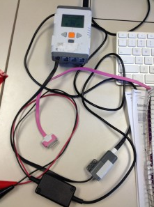
The solar cell is the little black box, which at first glance may look simple. However, after conducting the experiment I was able to see the way the cell actually worked and understand the complexity!
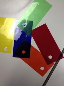
Our instructions were to hold the ruler up to the power cell and shine the light on the cell from varying distances above it. Then, with the help of LabView (thank god!), we were able to obtain the variances in data when we measured the light further away from the cell. We then did the same with the five different color panels we got from Professor Sonek. The panels looked like this:
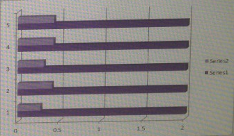
When we started, we did not see much variance in the data. This was concerning as the whole point of the lab was to compare the data. However, after a few trial runs, I began to understand how to correctly obtain the data. When we got a hang of the lab, we took data from shining the light at 8cm, 16cm, 21cm, and finally, 32cm. From these different distances, the effect of the distance of the light on the power cell was quite clear. When we began to add the colors, I guessed that they would not change much, however, I was sadly mistaken. The color panels actually did affect the data. I could not wrap my head around the fact that just because a panel was a different color, the power levels would be different! I would love to look more into this.
Anyways, our next task was to enter the data in excel and create graphs. This was perhaps the scariest part for me as I’m not an avid excel user and I really really really dislike graphs. After taking a deep breath and asking some questions, however, it all began to make sense to me. Maybe science isn’t so bad after all….
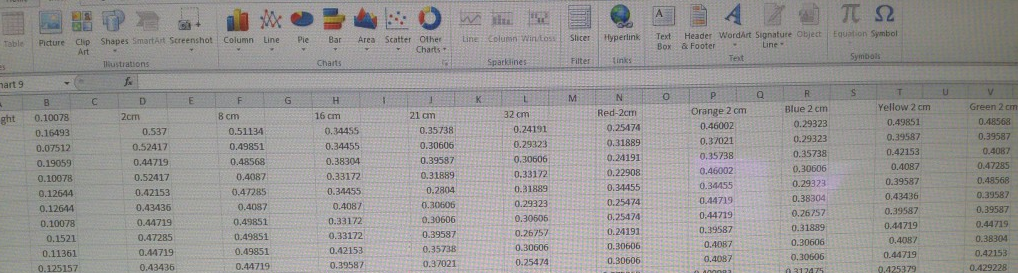
Our data appeared like this